When doing anything even vaguely related to quantitative genetics I would chose more missing data over more genotyping errors any day of the week. There are lots of approaches to making missing data less of a pain. The most straightforward of these is called imputation. Imputation essentially means using the genetic markers where you do have information to guess what the most likely genotypes would be at the markers where you don’t have any direct information on what the genotype is. This is possible because of a phenomenon known as linkage disequilibrium or “LD.” Both imputation and LD deserve their own entire write ups and they are on the list of potential topics for when I have another slow Sunday afternoon. For now the only thing you have to know about them is that, when information on a specific genetic marker is missing, it is often possible to guess with fairly high accuracy what that missing information SHOULD be. But when the information on a specific genetic marker is WRONG… well it’s usually a bit more of a mess (but I think the software solutions for this are getting better! Details at the end of the post.)
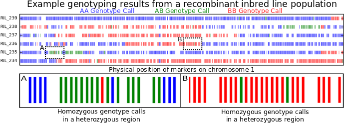
Figure 1: Genotype calls along chromosome 1 for six recombinant inbred lines (RILs).
To illustrate what genotyping errors look like without picking on anyone else, the figure at the top of this post is a little genotyping data from my own lab. I’m showing you data from only six recombinant inbred lines (or RILs). These lines were generated by crossing two parents, and then selfing the progeny for many generations. At the end, each individual line should be homozygous across almost its entire genome, with, on average, about equal portions of its genome coming from its father (red) and its mother (blue). Green regions are where an individual line still carrying one copy of the version of that piece of chromosome 1 from its mother and one copy of version of that same piece of chromosome 1 from its father. Places where the color changes as you move from left to right along an individual chromosome are called recombination breakpoints.
By looking at the number of recombination breakpoints between any two genetic markers across a larger population of RILs (~400 in this case) we can estimate how far away they are from each other. This is called “genetic distance” and it is measured in centiMorgans.* The plot above however is showing the positions of the markers on the chromosome based on their “physical distance” which is measured by just counting the number of DNA bases separating the two markers.** Because there are a LOT of total nucleotides on a chromosome, physical distance is often measured in kilobases or megabases. If there are no errors in the genetic map or the genome assembly, the order of genetic markers based on the genetic map and the physical map should be identical. However, the ratio of genetic distance to physical distance will vary across any given chromosome, so it’s not possible to calculate one directly from the other.
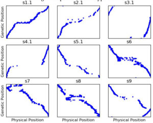
Figure 2: Genetic map generated from uncorrected genotyping by sequencing like data using ASMap****.
Counting recombination breakpoints is where genotyping errors start to cause serious problems. Look at box A and box B above. Box A contain should contain two recombination breakpoints, one where the beginning blue region switches to green and another where the green region turns back to blue. Box B shows a region that comes entirely from one parent in that particular RIL. However, each box contains two markers which were misgenotyped. If a computer counts recombination breakpoints, it’d count 6 in box A (blue to green, green to red, red to green, green to blue, blue back to green, green back to blue), and four in box B. As you can see, even a small proportion of incorrect genotype calls can start introducing a LOT of false recombination events into the dataset one would use to construct a genetic map. And the results of that are just plain ugly…
Figure 1 shows the genetic map**** we got when we first started using our genotype data to construct a genetic map. Remember that, while the ratio of genetic distance to physical distance can vary, the genetic and physical order of the markers should be the same. So s1.1 is reasonably okay (although there are still more out of order markers than I would like), but for a lot of the other chromosomes, the genetic and physical orders have lots of major disagreements.
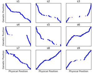
Figure 3: Genetic map constructed with ASMap with the same settings as Figure 2 but using SNP data after having run Genotype-Corrector
Many apparent*** genotype errors are easy for the human eye to spot, but with ~11,000 markers and ~400 RILs, no one has time to go through 4+ million datapoints to do the corrections manually. Enter Genotype-Corrector, a software package one of the students in my lab had developed during his masters to essentially do the same thing you or I do when we look at that graphic: “hey the genotype of marker in this line doesn’t agree with any of the markers around it, maybe it’s a mistake.” He volunteers to run Genotype-Corrector on this dataset, and afterwards I rebuilt the genetic map…. and the results were MUCH better.
Now there are things to be aware of with this approach. Essentially Genotype-Corrector and similar tools are borrowing information from the physical map (genome assembly) to correct errors in the data that is used to build a genetic map, so if there are mistakes in the genome assembly, this reduces your chances of catching them. In principle it should be possible to do the same type of error correction using only information on linkage between individual markers. LinkImpute already using a similar approach for imputation, but I don’t know of any software that uses the same principle for genotype error correction. If you do, please let me know in the comments below.
The manuscript for Genotype-Corrector is currently in review (I’ll update this post once it comes out somewhere), but the software and source code has already been released on github.
- Miao C, Fang J, Liang P, Zhang X, Schnable JC, Tang H. Genotype-Corrector: improved genotype calls for genetic mapping. (In Review)
*Named after a geneticist who worked of fruit flies a century ago.
**Easy to do if you have a well sequenced reference genome, more painful otherwise.
***There are other biological phenomena that could create the patterns observed in the two boxes of Figure 1, I just don’t have space to go into them here, this post is already going to be more than 1000 words.
****All genetic maps were constructing with ASMap, an R package that reimplements the MSTMap algorithm. I highly recommend it!