Functionless DNA changes more rapidly, functional DNA more slowly. This is one of the fundamental principles of comparative genomics. It’s why people look at the ratio of synonymous nucleotide changes to nonsynonymous nucleotide changes within the coding sequence of genes. It’s why the exons of two related genes will still have strikingly similar sequences after the sequence of the introns have diverged to the point where it’s impossible to even detect homology. It’s also a way to identify which parts of the noncoding sequence surrounding a set of exons are functionally constrained. The bits of noncoding sequence that determine where, and when, and how much, a gene is expressed are by definition, functional, and should diverge more slowly between even related species than the big soup of functionless noncoding sequence that the functional bits of a genome float in. These conserved, functional, noncoding sequences are called, unimaginatively, conserved noncoding sequences (CNS).*
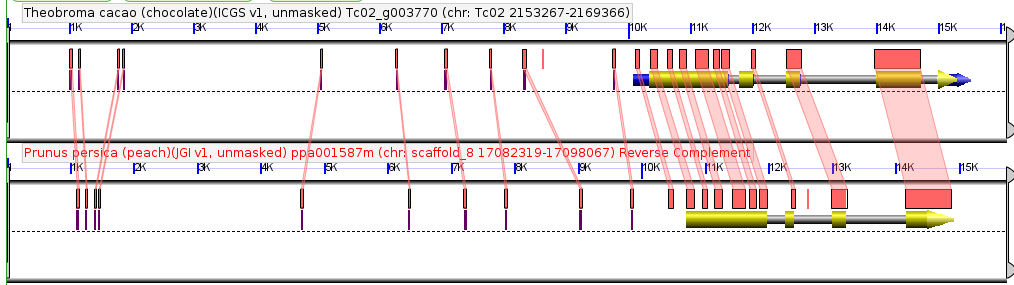
Comparison of a single syntenic orthologous gene pair in the genomes of peach and chocolate. Coding sequence marked in yellow, introns in gray, annotated UTRs in blue. Red boxes are regions of detectably similar sequence between the same genomic region in these two species. Taken from CoGePedia.
I’ve been playing with CNS since I first opened a command line window back as a first year grad student. The smallest CNS we’d consider “real” were 15 base pair exact matches between the same gene in two species. On the one hand, this seemed a bit too big, because I know lots of transcription factors bound to motifs as short as 6-10 base pairs long. On the other hand this seemed a bit too short because I’d see 15 base pair exact matches that couldn’t be real a bit too often (for example a match between a sequence in the intron of one gene, and the sequence after the 3′ UTR of another).
15 bp represented a compromise between the two concerns pushing in opposite directions. Then, in the fall of 2014, a computer science PhD student walked into my office and asked if I had any interesting bioinformatics problems he could work on. The result was a new algorithm (STAG-CNS) which was both more stringent at identifying conserved noncoding sequences and able identify shorter conserved sequences than was previously possible. It achieved both of these goals through the expedient of throwing genomes from more and more species at the problem.
The chance of two given 15 base pair sequences matching each other are 1/(4^15) which works out to almost exactly 1 in a billion. You’d think that would be enough to ensure any 15 base pair exact match between two genes represented a real conserved sequence. The problem is, that if I’m comparing one 10 kb sequence to another 10 kb sequence, there are 9,986 15 base pair sequences in each of those sequences, which means I’m making about 100 million comparisons. Suddenly those 1 in a billion odds of a match by chance alone don’t sound so reassuring. This is the curse of multiple testing, the special demon of all things genomics and bioinformatics.
What the algorithm that computer science student produced did** was to make it practical to look for the same sequences, in the same order (the fancy name for this is “conserved microsynteny”), in the promoters of three or more genes at once. If the odds of finding a given 15 base pair sequence twice by chance alone are on in a billion, the odds of finding it three times by chance were ~1/10^18 which is one in a quintillion, which is a number so big I had to look up what it was called. We could calculate the odds for even greater numbers “by chance” matches, but you get the idea.***
The manuscript below used showed that with only two species, the minimum conserved sequence with a false discovery proportion (FDP)**** less than 0.05 was actually 18 base pairs, not 15. However, it also showed that by throwing data from more species into the algorithm at the same time, it is possible to confidently identify shorter and shorted CNS while maintaining the same FDP. We stopped at six species, because that was the number of high quality sequenced grass genomes without Ft. Lauderdale issues we had to work with. At that point the algorithm was identifying sequences as short as 9 base pairs long that are absolutely conserved, in the same positions, in the promoters of that same gene in each species. Nine base pairs is still a bit long for a transcription factor binding site, but the algorithm should scale, so hopefully, when we have 10 or 20 high quality grass genomes (which isn’t all that far away), this same approach will be identifying individual, functionally constrained, transcription factor bindings sites.
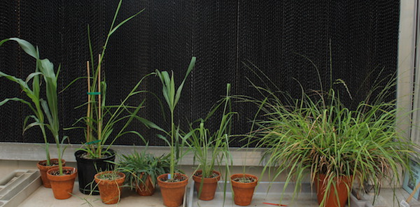
Still lots more interesting grass species left to sequence. From left to right: corn (sequenced), sorghum (sequenced), marsh grass (working on it), paspalum (working on it), dichanthelium (sequenced), foxtail millet (sequenced), urochloa (working on it), switchgrass (Ft. Lauderdale), chasmanthium (working on it). Used in this paper, but not pictured here: rice (sequenced), and brachypodium (sequenced). Photo credit: Daniel C.
*Except in the animal work where after a while they realized CNS also meant “Central Nervous System,” so they switched to calling them CNEs (Conserved Noncoding Elements).
**Using a combination of a suffix tree and a maximum flow algorithm, which I won’t even try to explain here, read the methods section of the paper if you are interested.
***All of this assumes DNA is purely random sequence with equal frequencies of all four nucleotides. There are obviously big problems with these assumptions, which is why in the paper we don’t use the predicted frequency of matches, but instead use permutation tests, where we compare the sequence around non-orthologous gene pairs where the only matches should be false positive ones, to identify the expected rate of false positives in our real data.
****
"false discovery proportion" <- based on the permutation tests we estimate how many false CNS we expect to find with ….
— James Schnable (@szintri) March 27, 2017
…a given set of parameters. Then look at the ratio between that number and the number discovered with the unpermuted data.
— James Schnable (@szintri) March 27, 2017
So FDP < 0.05 means we estimate less than 5% of the CNS discovered are false positives.
— James Schnable (@szintri) March 27, 2017